14.3 – Intersectoral Struggles over the Surplus

So far, we’ve assumed that the surplus that an economy produces goes entirely to the profits of the companies doing the production. For the sake of simplicity, we’ve assumed that workers are only paid a subsistence income, which we wrapped into the outlays of each sector, and implicitly we ignored other groups like government, charities, and so on. Now we can start to understand how the surplus is distributed between the various groups in the economy. We begin here by only considering the distribution between different sectors. In the next section, then, we’ll look at the distribution between classes. In each of these sections one of the most important things to understand is that who gets how much of the surplus is ultimately determined through power struggles between different groups–businesses, workers, and all the rest. Prices, profits, wages, and other dollar values are, in part at least, reflections of these contests.

Let’s use the previous section’s hypothetical economy, where steel was priced at $30 per ton, corn at $10 per ton, and each sector earned a profit rate of 93.75%. With these numbers in hand, we can rewrite the equations we’ve been working with just a little differently.

For the corn sector:

[latex](30 \text{ corn} \times $10 + 150 \text{ steel} \times $30)(1 + 0.9375) = 930 \text{ corn} \times $10[/latex]

And for the steel sector:

[latex](225 \text{ corn} \times $10 + 5 \text{ steel} \times $30)(1 + 0.9375) = 155 \text{ steel} \times $30[/latex]

These equations give us the incomes and revenues of each sector in dollar terms. Check for yourself that the left-hand side of each equation adds up to the right-hand side.

The left-hand sides of the two equations above give the sectors’ outlays multiplied by 1 plus the profit rates, expressed as decimals rather than percentages. That is to say, for each sector’s equation, the left-hand side shows the money invested times the amount of money the businesses in that sector brought in over and above their investment. The right-hand sides simply show the amount of money the sector generated by sale of its output. The two sides come out equal because prices are such that the output of each sector in dollar terms will be sufficient to earn those businesses the 93.75% rate of profit we calculated previously. We can write these equations more generically as:

[latex]\text{Total Costs} \times (1 + r) = \text{Total Revenues}[/latex]

Where r gives the markup over cost, which means the same as the profit rate. Now, it’s important to remember four points made previously before we begin to use this equation.

First, the total costs of a sector are determined in part by technology (for example, how much corn and steel is necessary to produce a ton of corn), in part by relative prices (how much corn costs relative to steel), and in part by how much output is being produced.

Second, the amount of output being produced is determined ultimately by businesses’ decisions about how much surplus to produce. In our model, we’re assuming that only the corn sector produces a surplus, so decisions about how much corn to produce as a surplus ultimately determine the rest of the quantities of corn and steel.

Third, relative prices are determined systematically and jointly with the determination of the surplus. This is just to say that if the economy is going to be able to continue to produce in the future–that is, if the economy is a going concern–and if profit rates are going to be equal across sectors, then these relative prices must hold. Corn doesn’t have to sell for $10, it could sell for $100 instead, but only if steel sold then for $300 instead of just $30.

And fourth, the profit rate (93.75% in our model) isn’t arbitrary, it’s the maximum rate of profit businesses can earn, given the decisions about how much to produce, which were already made. As you saw in the previous section, businesses can collectively increase their rate of profit by increasing their investments in production (provided there are additional unemployed resources to bring online), but once investments are made profits are effectively set in stone until the next period of production.

The third and fourth points above point the way to answering our big question of who gets how much of the surplus.

Although we’ve so far been thinking of the determination of relative prices as a mathematical problem to be solved, in real capitalist economies there’s no one putting pencil to paper to determine the appropriate relative prices of everything getting produced, and then dictating those prices to everyone in the economy. Real world prices are being set and changed all the time, in many different places, and by many different people–chiefly by corporate managers, not, as the orthodox approach would have you believe, by markets. The nature of these processes is neither collective nor mechanical (though, as chapter “The Megacorp” examines, businesses usually coordinate to some extent by various means). No, actual price determination is a complex system of power struggles, wrapped up in decisions about both how much surplus to produce and who will get what share of that surplus.

As an example, suppose steel companies in our hypothetical economy decided they wanted a bigger slice of the pie–that is, more profits. They’re going to (try to) get it by raising their prices. Now, assuming for the sake of argument that nothing has changed about the amount being produced, this changes the equations above in two ways: (1) the price of steel will go up as steel producers try to grab more money, and (2) the profit rates will change for both sectors. Let’s see how that works out.

Suppose the price of steel rises from $30 to $45 per ton. This gives us:

For the corn sector, changing only the price of steel and solving for the profit rate:

[latex](30 \text{ corn} \times $10 + 150 \text{ steel} \times $45)(1 + r_\text{corn}) = 930 \text{ corn} \times $10[/latex]

Which gives a profit rate (r_corn) of 31.9%

And for the steel sector:

[latex](225 \text{ corn} \times $10 + 5 \text{ steel} \times $45)(1 + r_\text{steel}) = 155 \times $45[/latex]

Which gives a profit rate (r_steel) of 181.8%

The result of the steel sector raising its prices is exactly what you would have expected: steel companies earn higher profits (a rate of 181.% versus 93.75% before), but at the expense of the corn companies (whose profit rate drops from 93.75% to 31.9%). Ask yourself what you might do if you were running one of these corn companies who just saw the cost of making farming implements (that is, the steel) rise dramatically.

If you said “I’d have to raise my prices” you’re doing well at thinking like a businessperson. To be sure, many businesses don’t like raising their prices if they can avoid it–doing so tends to upset their customers and, for many businesses at least, it’s best to keep the customer happy when possible. But when prices are up for the whole corn sector (that is, basically everyone, including your competitors, needs steel), pushing your profits down toward dangerously low levels, you’re probably going to have to raise your own prices to compensate.

And with our model we already know where corn prices need to go to get back to normal: as the previous section covered, to keep the economy viable and producing an equal profit rate between the sectors, steel needs to be priced at 3 times corn. So if steel now sells for $45 then the price of corn will need to increase from $10 to $15. This gives the following:

For the corn sector:

[latex](30 \text{ corn} \times $15 + 150 \text{ steel} \times $45)(1 + r_\text{corn}) = 930 \text{ corn} \times $15[/latex]

Which returns the profit rate (r_corn) back to 93.75%

And for the steel sector:

[latex](225 \text{ corn} \times $15 + 5 \text{ steel} \times $45)(1 + r_\text{steel}) = 155 \text{ steel} \times $45[/latex]

Which also returns the profit rate (r_steel) back to 93.75%

Notice that nothing actually changed in terms of the output produced or the inputs used. The steel sector continued to produce just enough steel for both sectors to keep producing into the future, and the corn sector continued to produce a surplus of 675 tons of corn. Indeed, once the corn companies responded to the higher steel prices by raising the price of corn, the relative prices returned to what they were in the beginning: steel sells for 3 times the price of corn. Really, the only thing that changed was the prices themselves.

This example demonstrates an important source of inflation: when price-setters decide they want more money but aren’t inclined to increase the actual output being produced, it will tend to simply raise all prices together. Fundamentally, this is because one business’ (or sector’s) output tends to be another business’ (or sector’s) inputs, so if everyone is going to stay in business (or the economy as a whole is to remain a going concern), then relative prices must be such that everyone can afford to pay for the inputs they need in the future with the money they’re making now. This, again, is what we mean by ‘prices are systematically determined’.

Understanding this can help us to explain certain historical periods of high inflation. Imagine, for instance, that instead of steel we had been considering oil. In the following breakout box, you’ll learn about an important component of the relatively high levels of inflation experienced in the U.S. during the 1970s.

Explaining the Inflation of the 1970s

Prior to the COVID-19 pandemic, the United States hadn’t seen a period of significant inflation for nearly four decades. Throughout the 1970s, however, inflation was a serious problem for the average American, even showing up in popular music such as Marvin Gaye’s 1971 classic “Inner City Blues”:

Inflation, no chance

To increase finance

Bills pile up sky high

Send that boy off to die

There are many explanations, some competing, some complementary, for the rapid increases in the price level from the late 1960s to the early 1980s, and economists don’t strictly agree on the most important causes. However, one cause of this inflationary period which nearly all economists recognize was the oil crises, first in 1973, and then again in 1979. The underlying geopolitics of these crises are too complex to cover here, but they chiefly involved political struggles in the Middle East. The price impacts of these crises can be seen clearly in Figure 1, below.

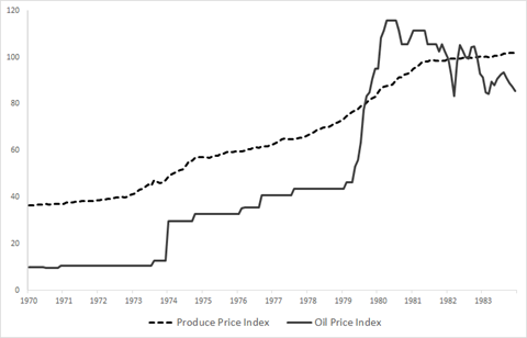
Along with the price of oil in figure 1, you can see clearly the impact on the overall price level, where the dashed line indicates the producer price index. Notice that, although prices were increasing prior to the 1973 oil embargo, they increased significantly faster following the embargo. The same pattern is evident again with the second oil crisis in 1979, and you can see at the end of the series that price increases slowed once oil prices started to fall, albeit modestly.

The pattern here isn’t hard to explain. Since oil is a vital input into much of what the American economy produces (from the gasoline that powers automobiles to the fertilizer to grow food), an increase in its price will ripple out into the prices of nearly everything else in the economy. Just like the example earlier in this section of the steel sector increasing the price of steel, when oil producers increase their prices, you can expect to see other sectors increasing their prices to keep themselves, and ultimately the economy as a whole, viable.

One final note: this explanation of inflation is a wholly different approach from the standard orthodox argument that sees inflation resulting from too much spending relative to output (see, for example, section “Pitfalls for Monetary Policy”). Here, we’re understanding inflation as a result, not of the interplay of abstract aggregate supply and demand curves, but rather of the concrete struggles for profits and the pricing decisions involved in those struggles between businesses, whole sectors, or even nations themselves.