
11.4 – Orthodox Economics and Policy Implications
Learning Objectives
By the end of this section, you will be able to:
- Discuss why and how orthodox economists measure inflation expectations
- Analyze the impacts of fiscal and monetary policy on aggregate supply and aggregate demand
- Explain the Phillips curve, noting its tradeoff between inflation and unemployment
- Identify clear distinctions between neoclassical economics and New-Keynesian economics
To understand the policy recommendations of the neoclassical economists, it helps to start with the New-Keynesian perspective. Suppose a decrease in aggregate demand causes the economy to go into recession with high unemployment. The New-Keynesian response would be to use government policy to stimulate aggregate demand and eliminate the recessionary gap. The neoclassical economists believe that the New-Keynesian response, while perhaps well intentioned, will not have a good outcome for reasons we will discuss shortly. Since the neoclassical economists believe that the economy will correct itself over time, the only advantage of a New-Keynesian stabilization policy would be to accelerate the process and minimize the time that the unemployed are out of work. Is that the likely outcome?
New-Keynesian macroeconomic policy requires some optimism about the government’s ability to recognize a situation of too little or too much aggregate demand, and to adjust aggregate demand accordingly with the right level of changes in taxes or spending, all enacted in a timely fashion. After all, neoclassical economists argue, it takes government statisticians months to produce even preliminary estimates of GDP so that politicians know whether a recession is occurring—and those preliminary estimates may be revised substantially later. Moreover, there is the question of timely action. The political process can take months to enact a tax cut or a spending increase. Political or economic considerations may determine the amount of tax or spending changes. Then the results of such policy changes may take even more time before changes in aggregate demand are observable through spending and production.
When economists and policy makers consider all of these time lags and political realities, active fiscal policy may fail to address the current problem, and could even make the future economy worse. The average U.S. post-World War II recession has lasted only about a year. By the time government policy activates, the recession will likely be over. As a consequence, the only result of government fine-tuning will be to stimulate the economy when it is already recovering (or to contract the economy when it is already falling). In other words, an active macroeconomic policy is likely to exacerbate the cycles rather than dampen them. Some neoclassical economists believe a large part of the business cycles we observe are due to flawed government policy. To learn about this issue further, read the following Clear It Up feature.
Why and how do economists measure inflation expectations?
People take expectations about inflation into consideration every time they make a major purchase, such as a house or a car. As inflation fluctuates, so too does the nominal interest rate on loans to buy these goods. The nominal interest rate is comprised of the real rate, plus an expected inflation factor. Expected inflation also tells economists about how the public views the economy’s direction. Suppose the public expects inflation to increase. This could be the result of a positive demand shock due to an expanding economy and increasing aggregate demand. It could also be the result of a negative supply shock, perhaps from rising energy prices, and decreasing aggregate supply. In either case, the public may expect the central bank to engage in contractionary monetary policy to reduce inflation, and this policy would result in higher interest rates. If, however, economists expect inflation to decrease, the public may anticipate a recession. In turn, the public may expect expansionary monetary policy, and lower interest rates, in the short run. By monitoring expected inflation, economists garner information about the effectiveness of macroeconomic policies. Additionally, monitoring expected inflation allows for projecting the direction of real interest rates that isolate for the effect of inflation. This information is necessary for making decisions about financing investments.
Expectations about inflation may seem like a highly theoretical concept, but in fact the Federal Reserve measures inflation expectations based upon early research conducted by Joseph Livingston, a financial journalist for the Philadelphia Inquirer. In 1946, he started a twice-a-year survey of economists about their expectations of inflation. After Livingston’s death in 1969, the Federal Reserve and other economic research agencies such as the Survey Research Center at the University of Michigan, the American Statistical Association, and the National Bureau of Economic Research continued the survey.
Current Federal Reserve research compares these expectations to actual inflation that has occurred, and the results, so far, are mixed. Economists’ forecasts, however, have become notably more accurate in the last few decades. Economists are actively researching how inflation expectations and other economic variables form and change.
The Discovery of the Phillips Curve
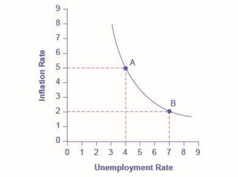
In the 1950s, A.W. Phillips, an economist at the London School of Economics, was studying the macroeconomic framework of the neoclassical synthesis. That framework implied that during a recession inflationary pressures are low, but when the level of output is at or even pushing beyond potential GDP, the economy is at greater risk for inflation. Phillips analyzed 60 years of British data and did find that tradeoff between unemployment and inflation, which became known as the Phillips curve. Figure 1 shows a theoretical Phillips curve, and the following Work It Out feature shows how the pattern appears for the United States.
The Phillips Curve for the United States
Step 1. Go to this website to see the 2005 Economic Report of the President.
Step 2. Scroll down and locate Table B-63 in the Appendices. This table is titled “Changes in special consumer price indexes, 1960–2004.”
Step 3. Download the table in Excel by selecting the XLS option and then selecting the location in which to save the file.
Step 4. Open the downloaded Excel file.
Step 5. View the third column (labeled “Year to year”). This is the inflation rate, measured by the percentage change in the Consumer Price Index.
Step 6. Return to the website and scroll to locate the Appendix Table B-42 “Civilian unemployment rate, 1959–2004.
Step 7. Download the table in Excel.
Step 8. Open the downloaded Excel file and view the second column. This is the overall unemployment rate.
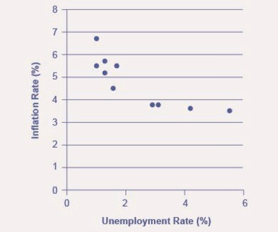
Step 9. Using the data available from these two tables, plot the Phillips curve for 1960–69, with unemployment rate on the x-axis and the inflation rate on the y-axis. Your graph should look like Figure 2.
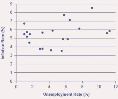
Step 10. Plot the Phillips curve for 1960–1979. What does the graph look like? Do you still see the tradeoff between inflation and unemployment? Your graph should look like Figure 3.
The Instability of the Phillips Curve
During the 1960s, economists viewed the Phillips curve as a policy menu. A nation could choose low inflation and high unemployment, or high inflation and low unemployment, or anywhere in between. Economies could use fiscal and monetary policy to move up or down the Phillips curve as desired. Then a curious thing happened. When policymakers tried to exploit the tradeoff between inflation and unemployment, the result was an increase in both inflation and unemployment. What had happened? The Phillips curve shifted.
The U.S. economy experienced this pattern in the deep recession from 1973 to 1975, and again in back-to-back recessions from 1980 to 1982. Many nations around the world saw similar increases in unemployment and inflation. This pattern became known as stagflation. (Recall from Chapter “The Aggregate Demand/Aggregate Supply Model” that stagflation is an unhealthy combination of high unemployment and high inflation.) Perhaps most important, stagflation was a phenomenon that New Keynesian economics had trouble explaining.
Orthodox economists have concluded that two factors cause the Phillips curve to shift. The first is supply shocks, like the mid-1970s oil crisis, which first brought stagflation into our vocabulary. The second is changes in people’s expectations about inflation. In other words, there may be a tradeoff between inflation and unemployment when people expect no inflation, but when they realize inflation is occurring, the tradeoff disappears. Both factors (supply shocks and changes in inflationary expectations) cause the aggregate supply curve, and thus the Phillips curve, to shift.
In short, we should interpret a downward-sloping Phillips curve as valid for short-run periods of several years, but over longer periods, when aggregate supply shifts, the downward-sloping Phillips curve can shift so that unemployment and inflation are both higher (as in the 1970s and early 1980s) or both lower (as in the early 1990s or first decade of the 2000s).
The Neoclassical Phillips Curve Tradeoff
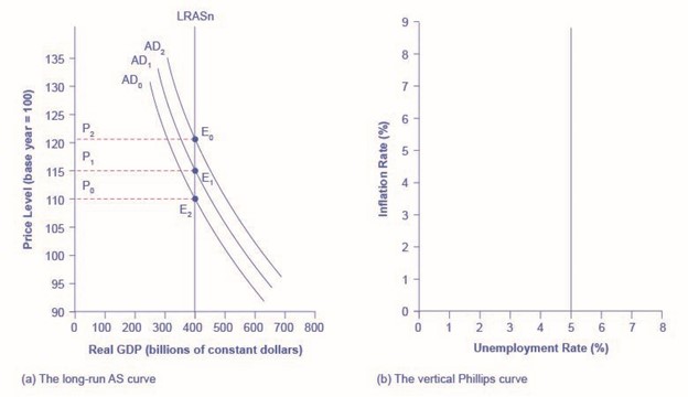
The Phillips curve can be derived from shifts in aggregate demand along the aggregate supply curve. The short run upward sloping aggregate supply curve implies a downward sloping Phillips curve; thus, there is a tradeoff between inflation and unemployment in the short run. By contrast, a neoclassical long-run aggregate supply curve will imply a vertical shape for the Phillips curve, indicating no long run tradeoff between inflation and unemployment. Figure 1 (a) shows the vertical AS curve, with three different levels of aggregate demand, resulting in three different equilibria, at three different price levels. At every point along that vertical AS curve, potential GDP and the rate of unemployment remains the same. Assume that for this economy, the natural rate of unemployment is 5%. As a result, the long-run Phillips curve relationship, in Figure 1 (b), is a vertical line, rising up from 5% unemployment, at any level of inflation. Read the following Work It Out feature for additional information on how to interpret inflation and unemployment rates.
Tracking Inflation and Unemployment Rates
Suppose that you are a macroeconomist in the future and have collected the following data for inflation and unemployment rates and recorded them in a table, such as Table 1. How do you interpret that information?
| Year | Inflation Rate | Unemployment Rate |
| 2050 | 2% | 4% |
| 2055 | 3% | 3% |
| 2060 | 2% | 4% |
| 2065 | 1% | 6% |
| 2070 | 1% | 4% |
| 2075 | 4% | 2% |
| 2080 | 5% | 4% |
Step 1. Plot the data points in a graph with inflation rate on the vertical axis and unemployment rate on the horizontal axis. Your graph will appear similar to Figure 2 below.
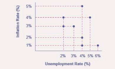
Step 2. What patterns do you see in the data of our hypothetical economy? You should notice that there are years when unemployment falls but inflation rises, and other years where unemployment rises and inflation falls.
Step 3. Can you determine the natural rate of unemployment from the data or from the graph? As you analyze the graph, it appears that the full employment lies at 4%. This is the rate that the economy appears to adjust back to after an apparent change in the economy. For example, in 2055 the economy appeared to have an increase in aggregate demand. The unemployment rate fell to 3% but inflation increased from 2% to 3%. By 2060, the economy had adjusted back to 4% unemployment and the inflation rate had returned to 2%. In 2065, the economy looks to have suffered a recession as unemployment rose to 6% and inflation fell to 1%. This would be consistent with a decrease in aggregate demand. By 2070, the economy recovered back to 4% unemployment, but at a lower inflation rate of 1%. In 2075 the economy again rebounded and unemployment fell to 2%, but inflation increased to 4%, which is consistent with a large increase in aggregate demand. The economy adjusted back to 4% unemployment but at a higher rate of inflation of 5%. Then in 2080, both unemployment and inflation increased to 5% and 4%, respectively.
Step 4. Do you see the Phillips curve(s) in the data? If we trace the downward sloping trend of data points, we could see a short-run Phillips curve that exhibits the inverse tradeoff between higher unemployment and lower inflation rates. If we trace the vertical line of data points, we could see a long-run Phillips curve at the 4% natural rate of unemployment.
The unemployment rate on the long-run Phillips curve will be the natural rate of unemployment. A small inflationary increase in the price level from AD0 to AD1 will have the same natural rate of unemployment as a larger inflationary increase in the price level from AD0 to AD2. The macroeconomic equilibrium along the vertical aggregate supply curve can occur at a variety of different price levels, and the natural rate of unemployment can be consistent with all different rates of inflation. The economist Milton Friedman (1912–2006) summed up the neoclassical view of the long-term Phillips curve tradeoff in a 1967 speech: “[T]here is always a temporary trade-off between inflation and unemployment; there is no permanent trade-off.”
In the New-Keynesian perspective, the primary focus is on getting the level of aggregate demand right in relations to an upward-sloping aggregate supply curve. That is, the government should adjust AD so that the economy produces at its potential GDP, not so low that cyclical unemployment results and not so high that inflation results. In the neoclassical perspective, aggregate supply will determine output at potential GDP, the natural rate of unemployment determines unemployment, and shifts in aggregate demand are the primary determinant of changes in the price level.
Fighting Unemployment or Inflation?
As we explained in chapter “Unemployment“, economists divide unemployment into two categories: cyclical unemployment and the natural rate of unemployment, which is the sum of frictional and structural unemployment. Cyclical unemployment results from fluctuations in the business cycle and is created when the economy is producing below potential GDP—giving potential employers less incentive to hire. When the economy is producing at potential GDP, cyclical unemployment will be zero. Because of labor market dynamics, in which people are always entering or exiting the labor force, the unemployment rate never falls to 0%, not even when the economy is producing at or even slightly above potential GDP. Probably the best we can hope for is for the number of job vacancies to equal the number of job seekers. We know that it takes time for job seekers and employers to find each other, and this time is the cause of frictional unemployment. Most economists do not consider frictional unemployment to be a “bad” thing. After all, there will always be workers who are unemployed while looking for a job that is a better match for their skills. There will always be employers that have an open position, while looking for a worker that is a better match for the job. Ideally, these matches happen quickly, but even when the economy is very strong there will be some natural unemployment and this is what the natural rate of unemployment measures.
The neoclassical view of unemployment tends to focus attention away from the cyclical unemployment problem—that is, unemployment caused by recession—while putting more attention on the unemployment rate issue that prevails even when the economy is operating at potential GDP. To put it another way, the neoclassical view of unemployment tends to focus on how the government can adjust public policy to reduce the natural rate of unemployment. Such policy changes might involve redesigning unemployment and welfare programs so that they support those in need, but also offer greater encouragement for job-hunting. It might involve redesigning business rules with an eye to whether they are unintentionally discouraging businesses from taking on new employees. It might involve building institutions to improve the flow of information about jobs and the mobility of workers, to help bring workers and employers together more quickly. For those workers who find that their skills are permanently no longer in demand (for example, the structurally unemployed), economists can design policy to provide opportunities for retraining so that these workers can re-enter the labor force and seek employment.
Neoclassical economists will not tend to see aggregate demand as a useful tool for reducing unemployment; after all, with a vertical aggregate supply curve determining economic output, aggregate demand has no long-run effect on unemployment. Instead, neoclassical economists believe that aggregate demand should be allowed to expand only to match the gradual shifts of aggregate supply to the right—keeping the price level much the same and inflationary pressures low.
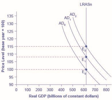
If aggregate demand rises rapidly in the neoclassical model, in the long run it leads only to inflationary pressures. Figure 3 shows a vertical LRAS curve and three different levels of aggregate demand, rising from AD0 to AD1 to AD2. As the macroeconomic equilibrium rises from E0 to E1 to E2, the price level rises, but real GDP does not budge; nor does the rate of unemployment, which adjusts to its natural rate. Conversely, reducing inflation has no long-term costs, either. Think about Figure 3 in reverse: as the aggregate demand curve shifts from AD2 to AD1 to AD0, and the equilibrium moves from E2 to E1 to E0. During this process, the price level falls, but, in the long run, neither real GDP nor the natural unemployment rate changes.
Fighting Recession or Encouraging Long-Term Growth?
Neoclassical economists believe that the economy will rebound out of a recession or eventually contract during an expansion because prices and wage rates are flexible and will adjust either upward or downward to restore the economy to its potential GDP. Thus, the key policy question for neoclassicals is how to promote growth of potential GDP. We know that economic growth ultimately depends on the growth rate of long-term productivity. Productivity measures how effective inputs are at producing outputs.
We know that U.S. productivity has grown on average about 2% per year. That means that the same amount of inputs produce 2% more output than the year before. We also know that productivity growth varies a great deal in the short term due to cyclical factors. It also varies somewhat in the long term. From 1953–1972, U.S. labor productivity (as measured by output per hour in the business sector) grew at 3.2% per year. From 1973–1992, productivity growth declined significantly to 1.8% per year. Then, from 1993–2014, productivity growth increased slightly to 2% per year. The neoclassical economists believe the underpinnings of long-run productivity growth to be an economy’s investments in human capital, physical capital, and technology, operating together in a market-oriented environment that rewards innovation. Government policy, according to these economists, should focus on promoting these factors.
Summary of Neoclassical and New Keynesian Macroeconomic Policy Recommendations
Neoclassical economists do not believe in “fine-tuning” the economy. They believe that a stable economic environment with a low rate of inflation fosters economic growth. Similarly, tax rates should be low and unchanging. In this environment, private economic agents can make the best possible investment decisions, which will lead to optimal investment in physical and human capital as well as research and development to promote improvements in technology.
In contrast, New-Keynesian economists argue there are benefits to be gained from “fine-tuning” the economy and, generally, see limited harm in advocating for policies designed to mitigate recessions. While New Keynesian economists accept the general precepts of the neoclassical perspective, when it comes to recessions, the New Keynesian position seems to say, “why wait?” Certainly, the long run can arrive on its own, but maybe policies can reduce the waiting time.
Summary of Neoclassical Economics and New-Keynesian Economics
Table 2, below, summarizes the key differences between the two orthodox macroeconomic visions.
| Summary | Neoclassical Economics | New-Keynesian Economics |
| Focus: long-term or short term | Long-term | Short-term |
| Prices and wages: sticky or flexible? | Flexible | Sticky |
| Economic output: Primarily determined by aggregate demand or aggregate supply? | Aggregate supply | Aggregate demand |
| Aggregate supply: vertical or upward-sloping? | Vertical | Upward-sloping |
| Phillips curve vertical or downward-sloping | Vertical | Downward-sloping |
| Is aggregate demand a useful tool for controlling inflation? | Yes | Yes |
| What should be the primary area of policy emphasis for reducing unemployment? | Reform labor market institutions to encourage full employment | Same as the neoclassical position with the exception of increasing aggregate demand to eliminate cyclical unemployment |
| Is aggregate demand a useful tool for ending recession? | At best, only in the short-run, temporary sense, but may just increase inflation instead | Yes |
Summary
Neoclassical economists tend to place their focus on factors that contribute to long-term growth. The concept of fighting recessionary conditions is generally minimized by neoclassical economists because they believe that recessions will fade in a few years, while long-term growth will ultimately determine the standard of living. They assume that the economy will tend to full employment, and therefore, see as mostly irrelevant those policies designed to mitigate the cyclical unemployment which is caused by recession.
Neoclassical economists also see no social benefit to inflation. With an upward-sloping New-Keynesian AS curve, inflation can arise because an economy is approaching full employment. With a vertical long-run neoclassical AS curve, inflation does not accompany any rise in output. If aggregate supply is vertical, then aggregate demand does not affect the quantity of output. Instead, aggregate demand can only cause inflationary changes in the price level. A vertical aggregate supply curve, where the quantity of output is consistent with many different price levels, also implies a vertical Phillips curve.
New-Keynesian economists, while generally in agreement with neoclassical theorists, are more apt than neoclassical theorists to encourage government policies that can offset recessionary, less than full employment, conditions. As such, inflationary conditions may be socially beneficial because an increase in inflation reflects an expanding economy producing rising employment.
the amount of total spending on domestic goods and services in an economy
the tradeoff between unemployment and inflation
an economy experiences stagnant growth and high inflation at the same time
a general and ongoing rise in price levels in an economy
unemployment closely tied to the business cycle, like higher unemployment during a recession
the unemployment rate that would exist in a growing and healthy economy from the combination of economic, social, and political factors that exist at a given time
