Numerical Simulation of Skydiving Motion*

Lawrence Davis

68 Numerical Simulation of Skydiving Motion*

Our goal for this chapter is to understand how we created the previously shown graphs of , , and of our example skydiver, even though the net force and acceleration changes throughout. We will use a that ties together just about everything we have learned so far in this unit to achieve this goal. We already know that the is zero and therefore the initial is zero. With no drag force in the first moment of the jump, the diver is in free fall and the acceleration is just g in the downward direction, or -9.8 m/s/s . We can then calculate the velocity after a short time interval $\Delta t$ as:

$\begin{equation*} \bold{v_1} = 0 + g\Delta t \end{equation*}$

We have made the that the acceleration during this interval was , even though it wasn’t, but if we choose a time interval that is very small compared to the time over which the acceleration changes significantly, then our result is a good . A time interval of one second will satisfy this condition in our case, so we now calculate the velocity at the end of the first one second interval:

$\begin{equation*} \bold{v_1} = 0 + g (1 \,\bold{s}) \end{equation*}$

Now that we have a velocity we can calculate the at the start of the second interval using our previously stated values for human , , and the standard value for air :

$\begin{equation*} \bold{F_{d,2}} = \frac{1}{2}C_d\rho A_x v_1^2 = \frac{1}{2}(1)(1.2\,\bold{kg/m^3})(0.45\bold{m^2})(.98 \,\bold{m/s})^2 = 0.259 \,\bold{N} \end{equation*}$

Now that we have a due to we can use to calculate the at the start of the second interval. We have only two forces, drag and gravity and we will use our previously stated skydiver of 80 kg:

$\begin{equation*} \bold{a_2} = \frac{\bold{F_{net}}}{m} = \frac{\bold{F_{d,2}}+\bold{F_g}}{m} = \frac{\bold{F_{d,2}}-mg}{m} = \frac{25.9 \,\bold{N}-(80 \,\bold{kg})(9.8\,\bold{m/s/s})}{80 \,\bold{kg}} =9.48 \,\bold{m/s/s} \end{equation*}$

Now we just continue this process of using acceleration and velocity values from the previous interval to calculate new velocity, drag force, and acceleration for next interval.

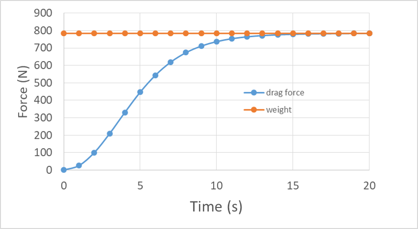
Using the data produced by the simulation we can graph the drag force. Showing the on the same graph we can see how the approaches the weight.

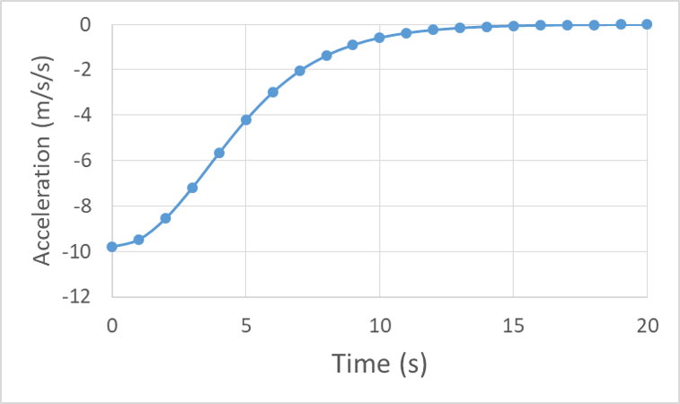
An example force vs. time curve for both drag and weight during a skydive. Weight is constant at 800 N. Drag starts at zero, increases with increasing slope (upward curvature), reaches an inflection point near 4 s, and continues to increase, but now with decreasing slope, and becomes indistinguishable from the weight value near 15 s.

We can also use the data to create motion graphs for the skydive and see that the gradually transitions from -9.8 m/s/s to zero as drag force increases.

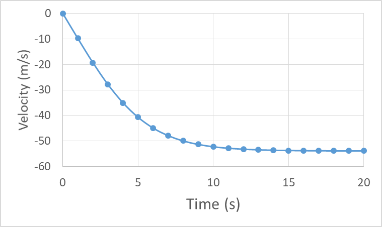
The acceleration vs. time curve replicates the shape of the force curve, but starts at -9.8 **m/s/s**, increases toward zero with increasing slope (upward curvature), reaches an inflection point near 4 s, and continues to increase, but now with decreasing slope, and becomes indistinguishable from zero near 15 s.

We see that is always negative and the is always increasing, but the becomes less steep because the is decreasing with time:

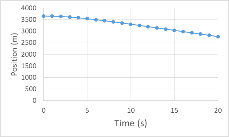
The velocity vs. time curve starts at zero and increases roughly linearly in the negative direction until near 4 s when it begins to level off and approach a constant 52 **m/s**.

Finally we can see that the graph eventually becomes linear as terminal velocity is reached. (Note that we have converted our of 12,000 ft to the equivalent 3660 m)

The position vs time curve starts at 3660 m and decreases toward zero with a negative and gradually steepening slope, nearing position 2750 m and slope of 52 **m/s** after 20 s.

License

Icon for the Creative Commons Attribution-NonCommercial-ShareAlike 4.0 International License

License

Share This Book