Basic Motion Graphs

Motion graphs are a useful tool for visualizing and communicating information about an object’s motion. Our goal is to create motion graphs for our example skydiver, but first let’s make sure we get the basic idea.

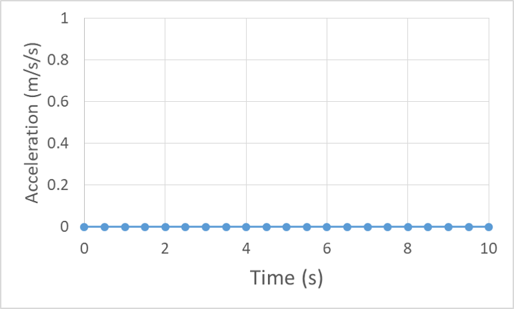
We will start by looking at the motion graphs of on object with an initial position of 2 m and constant velocity of 4 m/s. An object moving at constant velocity has zero acceleration, so the graph of acceleration vs. time just remains at zero:

The velocity is constant, so the graph of velocity vs. time will remain at the 4 m/s value:

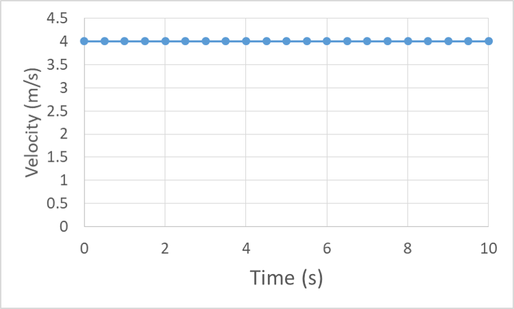
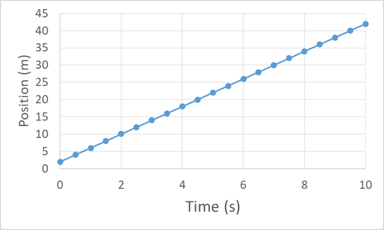
Velocity is the rate at which position changes, so the position v. time graph should change at a constant rate, starting from the initial position (in our example, 2 m). The slope of a motion graph tells us the rate of change of the variable on the vertical axis, so we can understand velocity as the slope of the position vs. time graph.

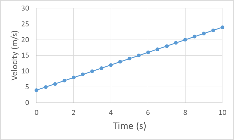
Now let’s look at motion graphs for an object with constant acceleration. Let’s give our object the same initial position of 2 m, and initial velocity of 4 m/s, and now a constant acceleration of 2 m/s/s. The acceleration vs. time remains constant at 2 m/s/s:

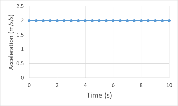
Acceleration is the rate at which velocity changes, so acceleration is the slope of the velocity vs. time graph. For our constant 2 m/s/s acceleration the velocity graph should have a constant  slope of 2 m/s/s:

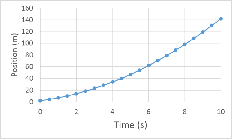
Finally, if the velocity is changing at a constant rate, then the slope of the position graph, which represents the velocity, must also be changing at a constant rate. The result of a changing slope is a curved graph, and specifically a curve with a constantly-changing slope is a parabolic curve, or a parabola.

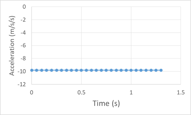
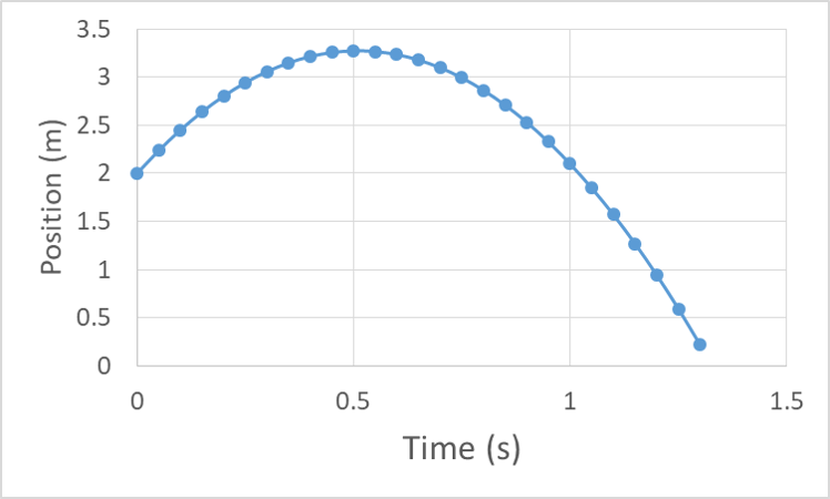
We haven’t made motion graphs for the situation of constant position because they are relatively unexciting. The position graph is constant at the initial value of position, the velocity graph is constant at zero and the acceleration graph is also constant at zero. Let’s end this section with some interesting graphs – those of an object that changes direction. For example, an object thrown into the air with an initial velocity of 5 m/s, from an initial position of 2 m that then falls to the ground at 0 m. Neglecting air resistance, the acceleration will be constant at  negative g, or -9.8 m/s/s.

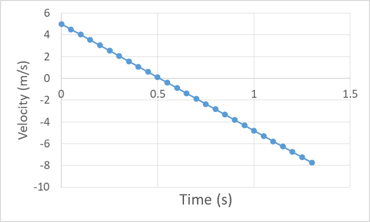
The velocity will be positive, but slowing down toward zero, cross through zero as the object turns around, and then begin increasing in the negative direction.

The position will increase as the object moves upward, then decrease as it falls back down, in a parabolic fashion because the slope is changing at a constant rate (acceleration is constant so velocity changes at a constant rate, so the slope of the position graph changes constantly).

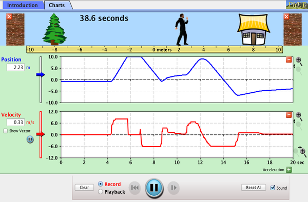
Check out this interactive simulation of a moving person and the associated motion graphs:

Everyday Example: Terminal Velocity

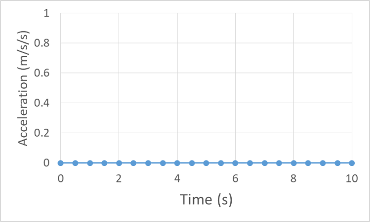
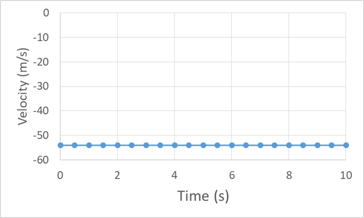
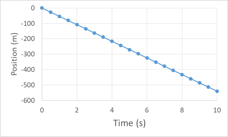
Let’s look at the motion graphs for our skydiver while they are at a terminal velocity of -120 MPH, which is about 54 m/s.  Let’s set our initial position for this analysis to be the position where they hit terminal velocity.

Acceleration is zero because they are at terminal velocity:

Velocity is constant, but negative:

And position changes at a constant rate, becoming more negative with time.

Everyday Example: Full Skydive

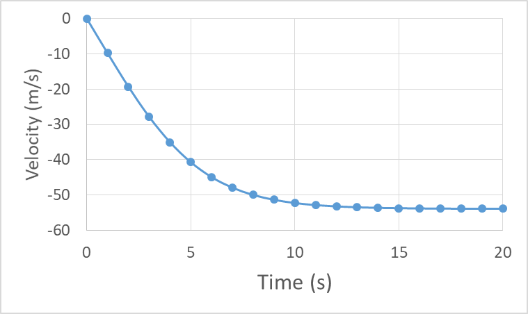
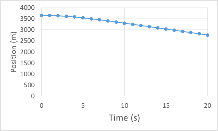
Now let’s look at the motion graphs for our skydiver prior to reaching terminal velocity, starting from the initial jump.

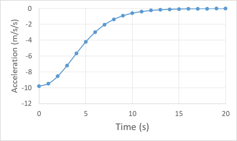The acceleration vs. time curve  starts at -9.8 m/s/s because in the first instant there is no drag force so the diver is momentarily in free-fall. As speed is gained, the drag force increases, cancelling out more of the weight, so the acceleration trends toward zero and becomes indistinguishable from zero near 15 s.